One of the main reasons why people can easily be re-identified in mobility data is because mobility patterns are highly unique. Consider your visited locations over the last few days, where did you go and when? E.g., you have been to your home, university, fitness studio, and your favorite supermarket. This combination of locations visited at specific timestamps will likely be unique for you, comparable to a fingerprint. An obvious choice of anonymization would be to coarsen space and time: e.g., not the exact location but a generalization to a, for example, 500x500m grid and not the exact timestamp but generalized to hour bins. Does this make your mobility trace (also trajectory) less unique?
De Montjoye et al. (2013)1 found that generalizing space and time decreases uniqueness (i.e., strengthens privacy) somewhat, but the influence of only adding a few more points to the trace is much higher and will make you quickly uniquely identifiable again. That means, even if a very coarse grid and coarse time windows are used, you will likely still be unique in a dataset if there are more than a few records of your whearabouts.
(To be clear, this scenario is NOT about retrieving exact locations one has visited, like retrieving the home location when only a coarse grid cell is provided. Instead, it is to evaluate the uniqueness of mobility traces, as unique traces can function as quasi-identifiers to re-identify individuals.)
A trace t is unique if no other trace within the dataset contains all of the spatio-temporal points (i.e., location visit at a certain time) that t is made of.
Montjoye et al.’s evaluation is based on mobile phone call detail records with spatial resolution equal to that given by the carrier’s antennas (this covers an area from 0.15 km2 per cell in the city to 15 km2 in rural areas) and a temporal granularity of one hour. They found, that only four spatio-temporal points are needed to uniquely identify 95% of users. When using a coarser resolution by combining 5 antennas to one spatial cell and using 5 h time windows, only about 49% of users are still identified uniquely with four spatio-temporal points. Though, adding 6 more points, so that there are 10 points available per user, makes the uniqueness jump back to about 85%.
Montjoye et al. even showed that it is possible to find a formula to estimate the fraction of unique traces (ε) given both, the spatial (v) and temporal (h) resolution of the data, and the number of points available to an outside observer (p). Note, that v (h) indicates how many antennas (hours) are clustered in one cell (time window), thus, the higher v (h) the coarser the resolution. The formula is as follows:
ε = α – (vh)β
The exact α and β (0 < β < 1) are parameters of the model, fit according to the specific dataset. α is only a dataset-dependent constant, at β we will have a closer look in a moment. First, we will understand the meaning of the the power-law dependency between ε and the spatial and temporal resolution (vh). As 0 < β < 1, the function (using some random α and β values for demonstration) looks somewhat like this:
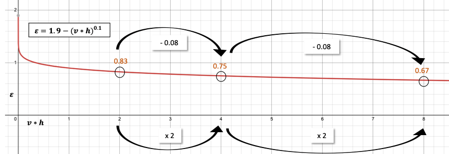
Note, that the displayed values are only for demonstration and are not generally applicable. They depend on the dataset and the number of available points per user (p), thus the values used for α = 1.9 and β =0.1 are randomly chosen.
Figure 1 shows, that if the resolution is divided by two (recall, an increase of x values means a reduction of granularity) the uniqueness of traces only decreases by a constant factor. This implies that privacy is increasingly hard to gain by lowering the resolution of a dataset.
What is also interesting to note, is that traces are more unique when one resolution is coarse (e.g., spatial dimension of v=10) but the other fine-granular (e.g., temporal dimension of h=1) compared to both dimensions being medium-grained (e.g, v=5 and h=5), as 1*10 = 10 but 5*5 = 25.
Next, we will have a closer look at the influence of adding more points (p), which is mitigated by β. The authors find that β is proportional to -p/100, e.g., given their dataset, β=0.157-0.007p. The exponent β decays linearly with p, thus, ε increases. See Figure 2, for an example how a value y increases linearly with a respective exponent (see Figure 2). First of all this means, as expected, the more points, the more unique the traces.
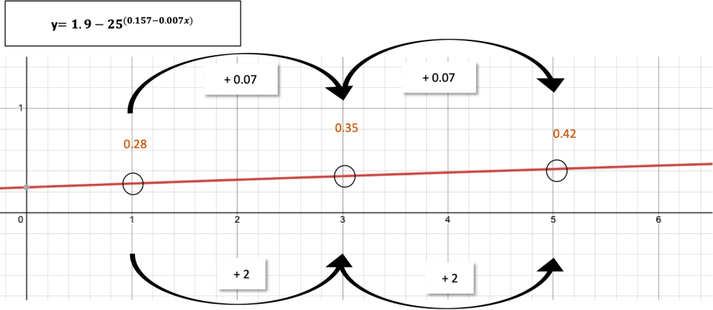
Second, while the resolution only impacts ε by a power-law dependency, the number of points have a linear influence. Thus, adding more points has a higher influence on the uniqueness than the resolution has. As the authors state: “A few additional points might be all that is needed to identify an individual in a dataset with a lower resolution.”
1de Montjoye, YA., Hidalgo, C., Verleysen, M. et al. Unique in the Crowd: The privacy bounds of human mobility. Sci Rep 3, 1376 (2013). https://doi.org/10.1038/srep01376

Leave a comment